We will take as an example the chi-square independence test (independence of two categorical variables).
Let’s take a variable X with four possible categories, and a variable Y with three categories. From a random sample, we get the following contingency table:
table = np.array([
    [6, 10, 20, 5],
    [12, 6, 22, 15],
    [20, 15, 4, 10]
])| X=1 | X=2 | X=3 | X=4 | |
|---|---|---|---|---|
| Y=1 | 6 | 10 | 20 | 5 |
| Y=2 | 12 | 6 | 22 | 15 |
| Y=3 | 20 | 15 | 4 | 10 |
The question that we ask with the chi-square independence test is: how likely is it to observe this table if the two variables are independent?
If the two variables are independent, then \(P(X | Y) = P(X)\) and \(P(Y | X) = P(Y)\). This means that the distribution of \(X\) for each row should match the overall distribution of \(X\), and likewise for the \(Y\). The overall distributions are given by the row and column totals:
| X=1 | X=2 | X=3 | X=4 | TOTAL | |
|---|---|---|---|---|---|
| Y=1 | 6 | 10 | 20 | 5 | 41 |
| Y=2 | 12 | 6 | 22 | 15 | 55 |
| Y=3 | 20 | 15 | 4 | 10 | 49 |
| TOTAL | 38 | 31 | 46 | 30 | 145 |
From these, we can compute the expected values of the contingency table under the independence hypothesis: \(e(X=i, Y=j) = \frac{n(X=i)*n(Y=j)}{n}\).
def compute_expected_frequencies(table: np.ndarray) -> np.ndarray:
    row_totals = table.sum(axis=1)
    column_totals = table.sum(axis=0)
    total = table.sum()
return np.outer(row_totals, column_totals)/total| X=1 | X=2 | X=3 | X=4 | TOTAL | |
|---|---|---|---|---|---|
| Y=1 | 10.7 | 8.8 | 13.0 | 8.5 | 41 |
| Y=2 | 14.4 | 11.8 | 17.4 | 11.4 | 55 |
| Y=3 | 12.8 | 10.5 | 15.5 | 10.1 | 49 |
| TOTAL | 38 | 31 | 46 | 30 | 145 |
Another way that we can get this table is through simulation. If we take the row and column totals as the frequency distribution of the two random variables, we can sample those variables \(N\) times and look at the simulated frequency table. If we repeat the experiment a large number of time, the “average frequency table” should be very close to the one we just computed:
def simulate_expected_frequencies(table: np.ndarray, n_repeats: int = 100_000) -> np.ndarray:
    total = table.sum()
    row_probs = table.sum(axis=1)/total
    column_probs = table.sum(axis=0)/total

    expected = np.zeros_like(table)

    for _ in range(n_repeats):
        X = np.random.choice(range(table.shape[1]), size=total, p=column_probs)
        Y = np.random.choice(range(table.shape[0]), size=total, p=row_probs)
        for x, y in zip(X, Y):
            expected[y, x] += 1
    return expected / n_repeats
Results after 100 000 random samplings:
| X=1 | X=2 | X=3 | X=4 | TOTAL | |
|---|---|---|---|---|---|
| Y=1 | 10.8 | 8.8 | 13.0 | 8.5 | 41 |
| Y=2 | 14.4 | 11.8 | 17.4 | 11.4 | 55 |
| Y=3 | 12.8 | 10.5 | 15.5 | 10.1 | 49 |
| TOTAL | 38 | 31 | 46 | 30 | 145 |
Now we know that the average value for the contingency table is what we expected, but how often do we deviate from this average value at least as much as in the observed table? To answer that, we need a measure of the deviation. For this test, the measure of deviation is the sum of squared differences, weighted by the expected values:
def deviation(expected: np.ndarray, observed: np.ndarray) -> float:
    return ((expected-observed)**2/expected).sum()
With this deviation measure, we can run the simulation again, but this time we don’t compute the average frequency table, we compute the deviation between the simulated table and the expected table. We can then look at how often this deviation is larger than or equal to the deviation of the observed table, and at what the distribution of deviations look like.
In pseudocode (see full code in pvalue-intuition.py
file):
Let T = observed table, n = repetitions
E := compute_expected_frequencies(T)
d := deviation(T, E)
deviations := []
do n times:
S := simulated_from_expected_values(E)
append deviation(S, E) to deviations
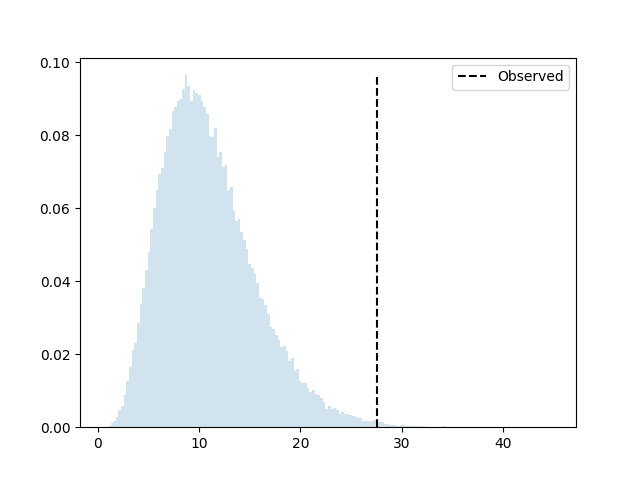
p_deviate_more := sum(d >= deviations)/nWhich will give us:
P(deviate more) = 0.00379
The dashed line is where our observed deviation is, and
P(deviate_more) is the sum of all the bins to the right of
it.
Now the theory of the chi-square independence test tells us that the deviation measure, under \(H_0\), follows a \(\chi^2\) distribution with \((p-1)(r-1)\) degrees of freedom, where \(p\) and \(r\) are the number of categories of \(X\) and \(Y\). Let’s put that distribution on top of our histogram:
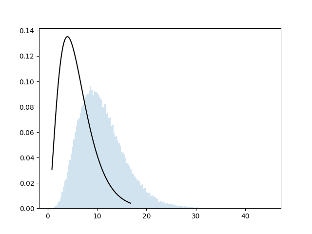
This doesn’t seem right. What’s the problem here?
The issue is that we computed “the deviation between the
simulated table and the expected table”. But that assumed that the
expected table is a known thing, even though we actually
computed it from the observed data. So our simulation is
incorrect: when we compute the “deviation”, we don’t know those
expected values, and we have to estimate them for each
simulated table. If we apply this correction, we change our
pseudocode to (see again full code in
pvalue-intuition.py):
Let T = observed table, n = repetitions
E := compute_expected_frequencies(T)
d := deviation(T, E)
deviations := []
do n times:
    S := simulated_from_expected_values(E)
    E2 := compute_expected_frequencies(S)
    append deviation(S, E2) to deviations
p_deviate_more := sum(d >= deviations)/n
And we now have:
P(deviate more) = 0.00013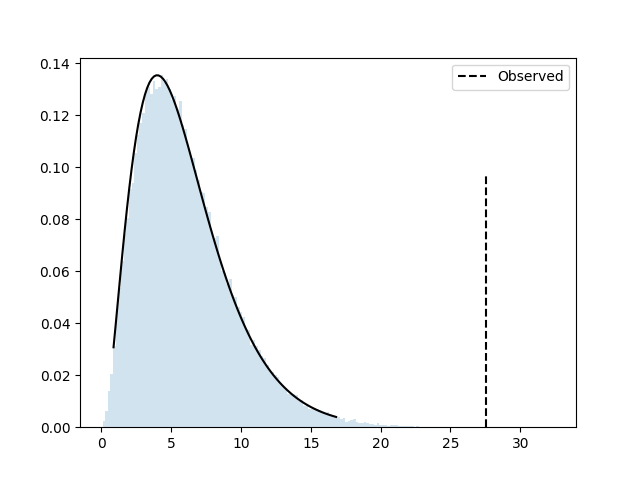
The simulated data follows the theoretical distribution very closely,
and P(deviate more) is the p-value that we would get
from the parametric test, for instance using
scipy.stats.chi2_contingency:
res = chi2_contingency(table)In this case, the theoretical computation gives us a p-value of
0.00011, very close to the 0.00013 from the
simulation.
The p-value in the chi-squared independence test is therefore the probability that, if the two variables are independent with probability distributions corresponding to those observed in the sample, we draw a contingency table at least as different from the expected table as the observed table.