The scipy library has a scipy.stats
module, which contains tons of classes and functions for using
different distributions. Here is a quick reference on how to use them
(although the documentation is well done, so you should probably read
that if you really need to use it!)
For the full code examples, check the
scipy-distributions.py file.
Let’s start by importing the package:
from scipy import statsThere are two different ways to use the distribution objects: we can first create an instance of the distribution and then call the methods you need, or you can call the methods in a static way. In the latter case, you’ll need to pass all the parameters of the distribution (e.g. mean, degree of freedom) at each method call.
Let’s see an example using the norm (Gaussian)
distribution and the rvs (random sampling) method:
# with instance
distrib = stats.norm(loc=5, scale=3) # N(5, 3**2)
sample = distrib.rvs(size=10)
[4.65890524 3.19035355 1.59434781 6.67730566 5.90081762 8.720739 3.85304134 4.99225494 3.03789302 5.92123052]# static
sample = stats.norm.rvs(loc=5, scale=3, size=10) # N(5, 3**2)[ 2.41477888 3.65682051 7.72652344 6.44591824 4.90958768 5.41533821 6.28139656 8.78508006 3.40068584 -1.60002674]Most distributions will have a loc and
scale parameter, which can be seen as “general” versions of
the mean and standard deviation, respectively. For the Gaussian
distribution, it is the mean and standard deviation, but other
distributions may have different ways of “shifting” and “scaling” the
function. For instance, stats.uniform (continuous uniform
distribution) uses loc for the minimum value, and
scale for the range, so
stats.uniform(loc=5, scale=3) will give a uniform
distribution with values between 5 and 8.
It is often very useful to be able to repeat experiments while being sure to get the same results. Being able to “fix” the randomness of the generators is therefore very useful.
scipy.stats uses the random_state parameter
as a way to ensure that you can get the same result everytime.
# with instance
distrib = stats.norm(loc=5, scale=3) # N(5, 3**2)
sample = distrib.rvs(size=10, random_state=1)
[ 9.87303609 3.16473076 3.41548474 1.78109413 7.59622289 -1.90461609 10.23443529 2.7163793 5.95711729 4.25188887]# static
sample = stats.norm.rvs(loc=5, scale=3, size=10, random_state=1) # N(5, 3**2)[ 9.87303609 3.16473076 3.41548474 1.78109413 7.59622289 -1.90461609 10.23443529 2.7163793 5.95711729 4.25188887]As we can see, we now got the same numbers in both calls to
rvs. Changing the random_state will give us a
new set.
The pdf function gives us the value of the
probability density function at the value x. By
varying x in a region of interest, we can plot the
probability density function. Using the same normal distribution as
before, let’s plot the function between \(\mu
- 3\sigma\) and \(\mu +
3\sigma\):
distrib = stats.norm(loc=5, scale=3)
x = np.linspace(5-9, 5+9, 100)

fig, ax = plt.subplots()
ax.plot(x, distrib.pdf(x),
        'r-', label=f'N(5,3²) pdf')
ax.legend()
These are sometimes the more confusing methods to use – and the most useful for statistical tests.
The CDF is the cumulative density function. So
cdf(x) will return \(P(X \leq
x)\), the “area under the curve” left of x.
distrib = stats.norm(loc=5, scale=3)
x = np.linspace(5-9, 5+9, 100)
cx = distrib.cdf(3)

fig, ax = plt.subplots()
ax.plot(x, distrib.pdf(x),
        'r-', label=f'N(5,3²) pdf')
ax.plot([3, 3], [0, distrib.pdf(3)], 'k--', label='x=3')
ax.text(0, 0, f'P(x <= 3) = {cx:.2f}', horizontalalignment='center')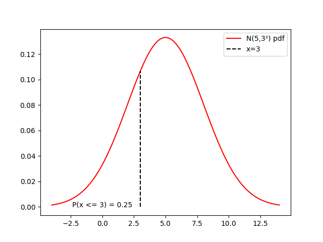
The PPF is the percent point function, which is the
inverse of the CDF. So ppf(x) will return \(v\) such that \(P(X \leq v) = x\), the “cutoff” point that
we need to get an area under the left curve of x. We can
check that it works as expected:
cx = distrib.cdf(3)
px = distrib.ppf(cx)
assert 3 == px
This is useful to find cutoff points for statistics: if we want a one-sided test at significance level \(\alpha = 0.05\) for a statistic that follows a distribution, we will have:
def significance_test(distrib, alpha: float, test_stat: float):
    cutoff = distrib.ppf(alpha)
    return test_stat < cutoff
This will return True if the test statistic in lower
than the cutoff, which means that it is outside the acceptance zone for
\(H_0\).
It is also useful for visualization: instead of manually setting the bounds of \(x\) as we’ve done before, which is not always easy depending on the distribution, we can plot between some percentiles of the CDF (e.g. 0.01 and 0.99). Let’s do it using another distribution, the \(\chi^2_{5}\):
distrib = stats.chi2(df=5)
fig, ax = plt.subplots()
x = np.linspace(distrib.ppf(0.01),
                distrib.ppf(0.99), 100)
ax.plot(x, distrib.pdf(x),
        'r-', label=f'pdf')
ax.legend()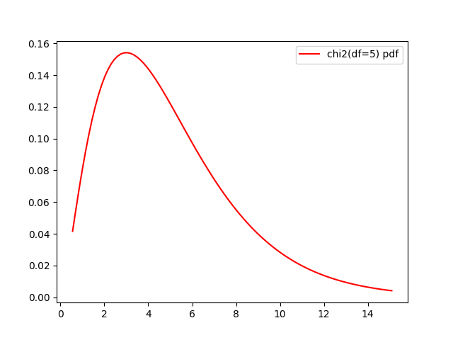
The SF is the survival function, which is simply
1-cdf. The ISF is its inverse.
They are useful for tests that look at the right side of the cutoff point when performing a significance test.
distrib = stats.norm(loc=5, scale=3)
x = np.linspace(5-9, 5+9, 100)
cx = distrib.sf(7)

fig, ax = plt.subplots()
ax.plot(x, distrib.pdf(x),
        'r-', label=f'N(5,3²) pdf')
ax.plot([7, 7], [0, distrib.pdf(7)], 'k--', label='x=7')
ax.text(10, 0, f'P(x >= 7) = {cx:.2f}', horizontalalignment='center')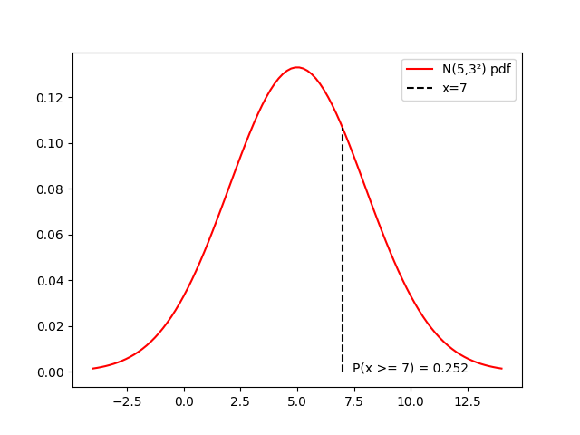
With the ISF and the PPF, we can find the cutoffs for the acceptance zone in a two-sided test.
def significance_test_ts(distrib, alpha: float, test_stat: float):
    cutoff_low = distrib.ppf(alpha/2)
    cutoff_high = distrib.isf(alpha/2)
    return test_stat < cutoff_high and test_stat > cutoff_low
Or show the acceptance zone on a plot:
distrib = stats.chi2(df=5)
alpha = 0.05

cutoff_low = distrib.ppf(alpha/2)
cutoff_high = distrib.isf(alpha/2)

x = np.linspace(distrib.ppf(0.01),
                distrib.ppf(0.99), 100)
fig, ax = plt.subplots()
ax.plot(x, distrib.pdf(x),
        'r-', label=f'chi2(df=5) pdf')
ax.plot([cutoff_low, cutoff_low], [0, distrib.pdf(cutoff_low)], 'k--')
ax.plot([cutoff_high, cutoff_high], [0, distrib.pdf(cutoff_high)], 'k--')
ax.text(4, 0, f'Acceptance zone', horizontalalignment='center')
ax.legend()
scipy continuous distributions have a method to estimate
the different parameters of a distribution from a sample (rv_continuous.fit).
For a normal distribution, this will just correspond to computing the mean and standard deviation:
true_distrib = stats.norm(loc=63, scale=7)
# random state for replicability
sample = true_distrib.rvs(size=30, random_state=0)

loc, scale = stats.norm.fit(sample)
print(loc, scale)
assert loc == sample.mean()
assert scale = sample.std()
66.09999513084222 7.57283929512745We can get something a little bit more interesting if we try to fit data to a \(\chi^2\) distribution. Let’s for instance get the sampling distribution of variances for 1.000 samples of size 30. This should follow a \(\chi^2_{29}\) distribution. Can we find that even if we only have the list of variances (so without knowing the degrees of freedom)?
# Generate the list of variances
variances = []
for i in range(1000):
        sample = true_distrib.rvs(size=30, random_state=i)
        variances.append(sample.var())

# Fit chi-squared
df, loc, scale = stats.chi2.fit(variances)
print(df, loc, scale)
An we can plot the probability density function of this estimated distribution against the histogram of variances:

Note: for a
chi2distribution, thelocandscaleparameters correspond to a shift and scaling of the distribution such that \(P(x \sim \chi^2_{df,loc,scale} \leq a) = \frac{P(\frac{x-loc}{scale} \sim \chi^2_{df,0,2} \leq a)}{scale}\)
estimated_distrib = stats.chi2(df=df, loc=loc, scale=scale)
x = np.linspace(estimated_distrib.ppf(0.01),
                estimated_distrib.ppf(0.99), 100)
y = (x-loc)/scale
p = estimated_distrib.pdf(x)
p2 = stats.chi2(df=df).pdf(y)/scale
assert np.allclose(p, p2)Another available method is interval, which gives us a
\(\alpha\)% confidence interval around
the median of a distribution. For the estimated \(\chi^2\) above, we can do:
c0, c1 = estimated_distrib.interval(alpha=0.95)And plot the results on the distribution:
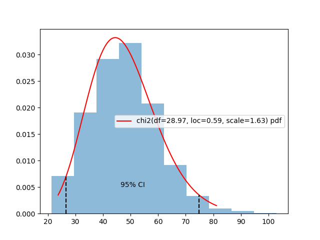
We could use this to redo the experiment in Module 2 of the course:
Example simulation: looking at how often the “true mean” is outside the CI using (a) a normal distribution, knowing the true variance, (b) a normal distribution, using the estimated sample variance, (c) a student distribution, using the estimated sample variance.
true_m = 63
distribution = stats.norm(loc=true_m, scale=7)
n = 20
oks_normal_true_s = []
oks_normal_s = []
oks_student_s = []
n_repeat = 100_000
for i in range(n_repeat):
X = distribution.rvs(n, random_state=i)
m = X.mean()
s = X.std(ddof=1)
cia = stats.norm.interval(loc=m, scale=7/np.sqrt(n), alpha=0.95)
cib = stats.norm.interval(loc=m, scale=s/np.sqrt(n), alpha=0.95)
cic = stats.t.interval(df=n-1, loc=m, scale=s/np.sqrt(n), alpha=0.95)

oks_normal_true_s.append(true_m >= cia[0] and true_m <= cia[1])
oks_normal_s.append(true_m >= cib[0] and true_m <= cib[1])
oks_student_s.append(true_m >= cic[0] and true_m <= cic[1])
print(f"Normal (true s): {sum(oks_normal_true_s)/n_repeat}")
print(f"Normal (estimated s): {sum(oks_normal_s)/n_repeat}")
print(f"Student (estimated s): {sum(oks_student_s)/n_repeat}")
Results:
Normal (true s): 0.95064
Normal (estimated s): 0.93627
Student (estimated s): 0.95097Sometimes, we have a sample that doesn’t follow a known shape, we we would still like to use the empirical distribution, and have access to the built-in PDF, CDF, PPF, random sample generation, etc. without having to recompute everything manually.
We can use for that the rv_histogram
class.
As an example, let’s create a distribution from the histogram of an image (using a Photo by J H on Pexels)
im = plt.imread(_FOLDER.joinpath(f"figs/pexels-jhawley-57905.jpg"))
bins = np.linspace(0, 256, 257)
hist, _ = np.histogram(im.flatten(), bins=bins, density=True)

distrib = stats.rv_histogram((hist, bins))
x = np.linspace(0, 256, 1024)
fig, axes = plt.subplots(1, 2, figsize=(10, 5))
ax = axes[0]
ax.imshow(im, vmin=0, vmax=255, cmap='gray')
ax.axis('off')
ax = axes[1]
ax.hist(im.flatten(), bins=bins, density=True, alpha=0.5)
ax.plot(x, distrib.pdf(x),
        'r-', label=f'pdf')
ax.legend()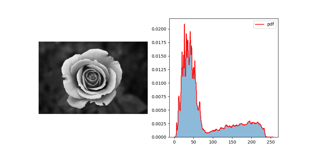
We can then use the standard methods for continuous distributions,
such as the cdf to get the cumulative probability, or
rvs to get a random sample drawn from this
distribution:
distrib.rvs(size=10)[ 47.45698774 15.81867229 53.0402298 41.74964717 194.33798125 53.30346215 19.84414427 165.42689923 40.16263265 11.27303173]fig, ax = plt.subplots()
ax.plot(x, distrib.cdf(x), 'r-', label=f'cdf')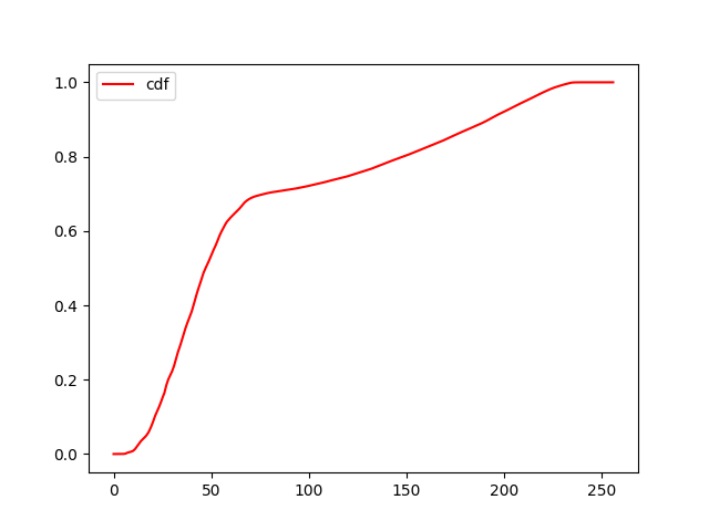
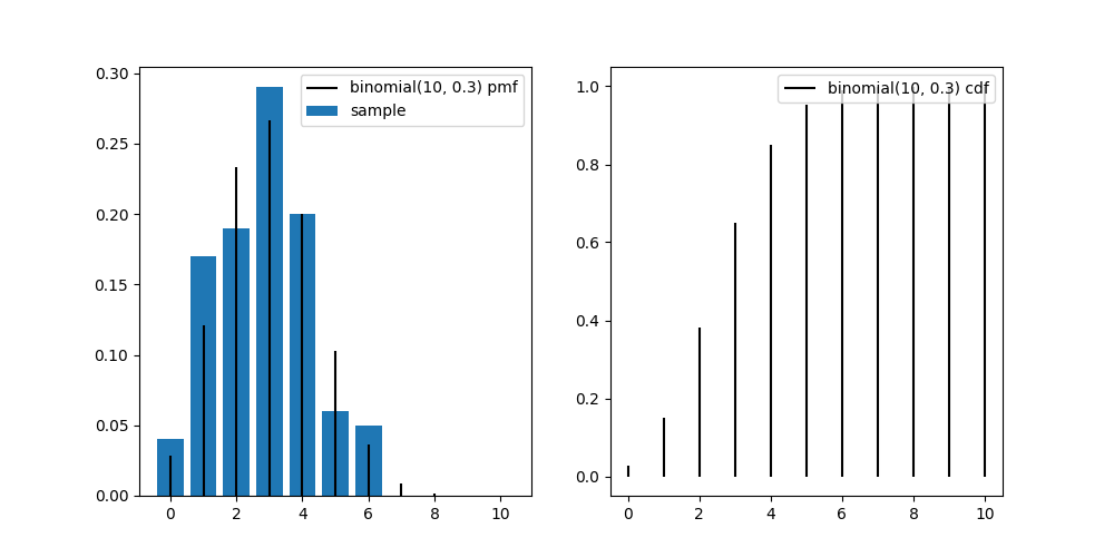
Similarly to the continuous functions, scipy.stats also
provide discrete distributions, such as the Binomial
distribution.
The main difference with the continuous distributions is that instead of a PDF, we have a PMF – probability mass function – which only has nonzero probability for integer values.
Otherwise, we can use the same methods as with continuous distributions, to generate random samples and use the CDF, PPF, etc.
n = 10
distrib = stats.binom(n=n, p=0.3)
sample = distrib.rvs(size=100, random_state=0)

x = range(n+1)
fig, axes = plt.subplots(1, 2, figsize=(10, 5))
ax = axes[0]
ax.bar(x, [(sample==v).sum()/len(sample) for v in x], label='sample')
ax.vlines(x, 0, distrib.pmf(x), colors='k', label='binomial(10, 0.3) pmf')
ax.legend()
ax = axes[1]
ax.vlines(x, 0, distrib.cdf(x), colors='k', label='binomial(10, 0.3) cdf')
ax.legend()